


Intro
Runtime procedural textures (not baked into bitmaps) have a minuscule memory footprint and can be customized at runtime, which are great features. However controlling aliasing during rendering can be difficult, unless there's some intermediate procedural-to-bitmap cache that facilitates prefiltering (like in Renderman's RtxPlugin for example). In the absence of such a system, one can always selectively supersample the texture as an numerical approximation to filtering, which reduce the aliasing to some degree. However, some procedural patterns can be analytically filtered just by the simple nature of their construction. That means that some special procedural functions can be rendered without aliasing, at least when in isolation. Now, the integral of function composition is generally not the composition of the integrals, meaning, a filtered complex shading network is not the same as a non-filtered network of the filtered elements it is made of. However in practice we can analytically filter these patterns individually and still get a reasonably band-limited results out of the network (probably slightly over-blurred).
Actually, while "band-limiting" doesn't substitute proper filtering, it is a valid alternative approach to the problem of aliasing. Anybody doing procedural content has implemented band-limiting at some point, either in the form of geometrical or shading/texturing static LODs, or through direct manipulation of the construction of the procedural detail. The technique is old as computer graphics and even the Renderman Shading Language documentation talks about it. But in this article we'll go through a short journey to rediscovering it so we can employ it more often in our procedural patterns.

Left: raw fBM. Right: band-limited fBM. Source+demo: https://www.shadertoy.com/view/3tScWd
From filtering to band-limiting cos(x)
Cos(x) (or Sin) is one of the most popular functions to generate procedural content since it's periodic, smooth and very fast to evaluate (in modern hardware). A cosine wave also has the advantage that it can be analytically integrated, so we can use the same filtering technique we used for square waves during pattern sampling/evaluation. Basically, given a cosine, we first need to know how much domain it actually covers across the a given pixel's footprint. Let's call that amount w, and use it to filter/convolve/integrate the cosine with a filter width (or kernel size) equal to w in order to compute the average value of the cosine within that pixel:
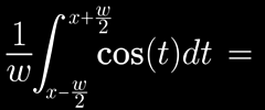

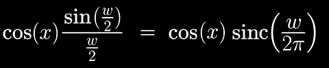
As we see, it so happens that filtering a cosine wave with a box filter is the same as multiplying it with a sinc() function, which comes as no surprise if you understand digital signal processing. A triangular kernel also produces an analytical solution, but for the purposes of today's exercise we'll stick to the box filter.
Now, let's apply this directly to a procedural pattern, for example a cosine based color texture that we deformed through some domain distortion, like this one:

Naive vs filtered cosines. Source+Demo: https://www.shadertoy.com/view/wtXfRH
On the left side of the image you see a naive implementation of the procedural texture (based on a series of cosine based color layers), where cos() is called directly, as you would normally do. On the right is the filtered version where each cosine function has been replaced with the filtered-cosine function we just deduced through our fancy maths. Let me show you the code for the naive texture implementation:
// palette
vec3 getColor( in float t )
{
vec3 col = a0;
col += a1*cos(k2PI*t* w1 + k1);
col += a2*cos(kTAU*t* w2 + k2);
col += a3*cos(k2PI*t* w3 + k3);
col += a4*cos(kTAU*t* w4 + k4);
col += a5*cos(k2PI*t* w5 + k5);
col += a6*cos(kTAU*t* w6 + k6);
col += a7*cos(k2PI*t* w7 + k7);
col += a8*cos(kTAU*t* w8 + k8);
return col;
}
a0 = vec3(0.4,0.4,0.4);
a1 = vec3(0.0,0.8,1.1), w1 = 1.1;
a2 = vec3(0.3,0.4,0.1), w2 = 3.1;
a3 = vec3(0.1,0.7,1.1), w3 = 5.1;
a4 = vec3(0.2,0.8,1.4), w4 = 9.1;
a5 = vec3(0.2,0.6,0.7), w5 = 17.1;
a6 = vec3(0.1,0.6,0.7), w6 = 31.1;
a7 = vec3(0.0,0.5,0.8), w7 = 65.1;
a8 = vec3(0.1,0.4,0.7), w8 = 115.1;

So, if supersampling the texture is not an option, we might have to consider removing some of the higher frequency cosines (say w7 and w8) in order to remove aliasing. And indeed that would remove the aliasing, but we'd also remove visual detail from the areas of the image which looked fine to begin with, which is not good. So, here's where the analytic filtering we just developed comes in handy because it does filter detail selectively, only removing high frequency content where it offends the image quality. As a result it produces a beautiful (smooth and stable) render as you can see on the right side of the picture. The nicest thing of it all is that the code is trivial - just a direct translation of the math we deduced - and it is a direct replacement for regular cos():
float fcos( in float x )
{
float w = fwidth(x);
return cos(x) * sin(0.5*w)/(0.5*w);
}
In terms of implementation, you could create a second version of this function where the filter width is manually passed to fcos(), which can become handy in some situations (more on that later). Also in terms of implementation, if you decided to optimize it, you might end up with something like the following:
float fcos( in float x )
{
float w = fwidth(x);
return cos(x) * smoothstep( k2PI, 0.0, w );
}

Now, besides some potential speed improvement, the smoothstep version will probably start giving you some ideas to extend this technique further. After all, what the smoothstep is effectively doing is smoothly deactivating the cosine wave (zeroing it out) when the size of a 2π cycle is smaller than a pixel. Basically, we replaced filtering by band-limiting (cancelling frequencies too high to be sampled without aliasing). So, under this light, it seems natural to apply the same deactivation treatment to other procedural oscillating functions which are not necessarily easy to integrate/filter, say, noise functions.
Band limiting noise
From this path of reasoning, the idea of approximating filtered noise by blending it towards zero based on the ratio wavelength-to-filter-width is inevitable, almost forced on us. You'll find it documented in old computer graphics manuals of a few decades ago. But despite being old and simple, it produces relatively acceptable results. Let's take for example a traditional FBM construction where we accumulate noise waves, and improve it by using a filtered noise primitive instead:
float fbm( in float x )
{
float f = 1.0;
float a = 0.5;
float t = 0.0;
for( int i=0; i<nOcts; i++ )
{
t += a*noise(f*x);
f *= 2.01;
a *= 0.50;
}
return t;
}
float ffbm( in float x )
{
float w = fwidth(x);
float f = 1.0;
float a = 0.5;
float t = 0.0;
for( int i=0; i<nOcts; i++ )
{
t += a*fnoise(f*x,w);
f *= 2.01;
w *= 2.01;
a *= 0.50;
}
return t;
}
float fnoise( in float x, in float w )
{
return noise(x)*smoothstep(1.0,0.5,w);
}
First, the code above can be trivially generalized to 2D and 3D, at least for isotropic band-limitation, by compute the length or the largest component of fwidth(). For anisotropic filtering, fnose() would have to be changed to something smarter.
Secondly, the choice of 0.5 and 1.0 in the smoothstep are a bit arbitrary, all that matters is that we attenuate things that oscillate more than once per pixel (in theory, half-times per pixel, according to Nyquist).
Thirdly, the propagation of the filter width w needs to be in synch with the doubling of the frequency, naturally. If the domain of noise() was deformed in other (potentially non-linear) ways, we would need to make sure the filter width shape was preserved as well (we'd need to track the multiple partial derivatives of the deformation). Related:
Lastly, I could have decided to not pass w to fnoise() and instead compute it inside the noise implementation, like with did with fcos(). However in this example above I wanted to show how to compute the filter width only once, in the callee, and then propagate it down the cascade of noise octaves; which could potentially be faster.
Now, as a post-implementation observation, we could argue that all we are doing is removing detail from our procedural content based on distance. And that can be true, but mischaracterizes the deeper relationship between pixel-footprint and the signal we are sampling. But, it is true that it is a valid simplified interpretation, although it is a valid one only in some scenarios. For example, indeed we often use that simple heuristic when creating massive procedural landscapes. In such applications, the lowest hanging fruit in the pursue of performance and antialiasing is the deactivation of octaves of procedural noise based on distance. For an fBM terrain in particular that happens in a logarithmic fashion since detail diminishes linearly with distance (due to perspective). So oftentimes, one attenuates and discards noise calls. But, this approach becomes less effective when there are space warping or other deformations dilating or expanding space in the mix, which is often employed to enrich procedural terrains with interesting geographical features. The reason the distance heuristic is less effective then is that the relation between distance and filter width is no longer just inverse-linear. Indeed different amounts of texture/noise space will fit in a single pixel depending on how much the domain was stretched/dilated. So, in those cases we need to compute the exact filter width, to prevent over and under-filtering. Now, you can compute that filter width analytically by propagating domain expansion/contraction through the chain rule of the Jacobians if each one of the deformations. Or you can also just rely on the filter width computed automatically for you in your hardware or software rendering package (say fwidth() in GLSL or filterregion in Renderman), which is easy and works really well in most situations.
Conclusion
While band-limiting is not a true replacement for actual filtering (whether analytical, supersampled or mipmap based), it is definitely better than not doing anything about aliasing, and in some cases it actually is a good solution for noise based functions. For cosine functions one can do this exactly as well. The following below is a live example of that actually; click and scroll the mouse to see the difference between filtering and not, and on the title to see the source code. .