


Intro
Voronoi patterns are widely used in computer graphics for procedural modelling and shading/texturing. However, when used for shading, one has to be extra careful because voronoi signals are discontinuous by definition and therefore difficult to filter. That's why normally these patterns are supersampled and baked into textures. There are other reasons to prefer baking over procedural evaluation, like filtering under minification, which is a problem with all procedural signals actually. Yet, i'd like to give the voronoi pattern a second chance as a procedural primitive, just for the sake of playing around. So, lets see if we can fix that ugly discontinuity at its source.
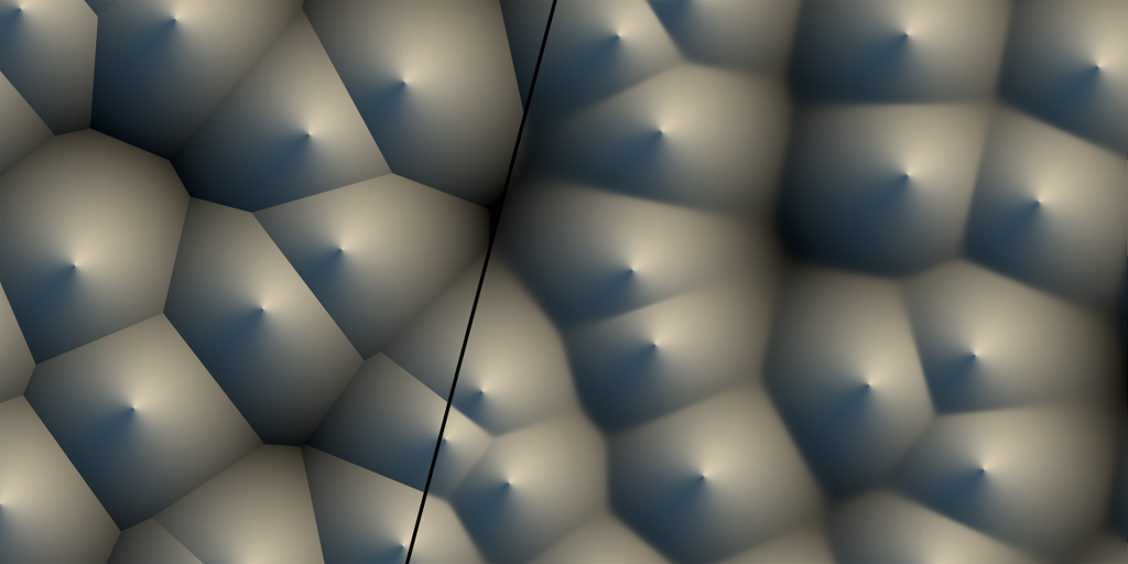
Regular voronoi on the left, smooth voronoi on the right
A reminder of where we are
Usually a voronoi function returns many signals, like the distance, id and position of the closest features. To keep things simple, though, lets write a very simple and classic voronoi pattern implementation this time:
float voronoi( in vec2 x )
{
ivec2 p = floor( x );
vec2 f = fract( x );
float res = 8.0;
for( int j=-1; j<=1; j++ )
for( int i=-1; i<=1; i++ )
{
ivec2 b = ivec2( i, j );
vec2 r = vec2( b ) - f + hash2f( p + b );
float d = dot( r, r );
res = min( res, d );
}
return sqrt( res );
}
As expected, the domain is partitioned in a grid, the cell in which the current shading point x lays is determined, the set of 3x3 cells centered in it is scanned, a pseudo-random point is generated in side each of these 9 cells, and the distance from x to the closest such point is recorded. So far so good.
Before continuing, it might be worth noting that there's a nice trick in this code above. Most implementations out there suffer from precision issues, because they generate their random points in "domain" space (like "world" or "object" space), which can be arbitrarily far from the origin. One can solve the issue by moving all the code to higher precision data types, or by being a bit clever. My implementation does not generate the points in "domain" space, but in "cell" space: once the integer and fractional parts of the shading point are extracted and therefore the cell in which we are working identified, all we care about is what happens around this cell, meaning we can drop all the integer part of our coordinates away all together, saving many precision bits. In fact, in a regular voronoi implementation the integer parts of the point coordinates simply cancel out when the per cell feature points are subtracted from the shading point. In the implementation above, we don't even let that cancelation happen, because we are moving all the computations to "cell" space. This trick also allows one to handle the case where you want to voronoi-shade a whole planet - one could simply replace the input to be double precision, perform the floor() and fract() computations, and go floating point with the rest of the computations without paying the cost of changing the whole implementation to double precision. Of course, same trick applies to Perlin Noise patterns (but i've never seen it implemented nor documented anywhere).
Fixing the issue
Back to our discontinuity issue. The problem with the voronoi pattern is of course the min() operation, that's where the discontinuity is introduced. Therefore, the idea today is to replace that min() operator with something that is similar enough, but continuous. If you think about it, the concept here is that we have a set of 9 points from which we are going to pick only one - the closest. So, what if instead of picking only one point we do actually pick them all but give to the closest one the most relevance, yet not full importance, such that as we move over the domain and new points become closer to our shading point we can smoothly transfer importance from the old closest point to the new one. In other words, what if instead of picking the distance to the closest point, we do a weighted average of the distances to all the points, in a way that it all resembles a min() operation so that we preserve the well known voronoi look.
This can be done in many ways of course. For example, one can use the inverse of the distance raised to a big power as a closeness factor, then add them all together and undo the inversion and the power in the end, in the hope that the closest distance will gain over the others in relevance. This works pretty well, but can have precision issues.
Another alternative is to use a quickly decaying exponential of the distance. This behaves nicer and provides a very intuitive control for the smoothness of the function, the downside being that it needs one extra square root in the inner loop.
These are implementations of both ideas:
float smoothVoronoi( in vec2 x )
{
ivec2 p = floor( x );
vec2 f = fract( x );
float res = 0.0;
for( int j=-1; j<=1; j++ )
for( int i=-1; i<=1; i++ )
{
ivec2 b = ivec2( i, j );
vec2 r = vec2( b ) - f + hash2f( p + b );
float d = dot( r, r );
res += 1.0/pow( d, 8.0 );
}
return pow( 1.0/res, 1.0/16.0 );
}
float smoothVoronoi( in vec2 x )
{
ivec2 p = floor( x );
vec2 f = fract( x );
float res = 0.0;
for( int j=-1; j<=1; j++ )
for( int i=-1; i<=1; i++ )
{
ivec2 b = ivec2( i, j );
vec2 r = vec2( b ) - f + hash2f( p + b );
float d = length( r );
res += exp2( -32.0*d );
}
return -(1.0/32.0)*log2( res );
}
To ensure these functions are perfectly and mathematically derivable/smooth one would need to window the distance decaying function with a smoothstep or something. While super easily doable, the strong decay of the exponentials makes it numerically continuous anyway. Depending on the falloff, though, you might want to extend the search neighborhood to a 5x5 grid, perhaps.
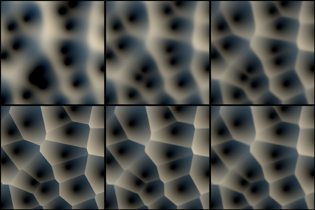
Lastly, this is the effect on the continuity of the pattern when varying the distance falloff in the exponential smooth voronoi. Top left: falloff=4, top center falloff=8, top right falloff=16, bottom right falloff=32, bottom center falloff=64, bottom left classic voronoi for reference.
Alternatives
One of the issues with the smooth minimums proposed above, is that they use relatively expensive exponential or power functions. The upside is that both produce associative smooth minimum, which means that the final value for the smooth minimum doesn't depend on the order in which the cells in the voronoi are processed. In reality, cheaper alternatives such as the polynomial smooth minimum described in this other article will most likely end up in your implementation. Such a polynomial smooth minimum is no longer associative, but in practice I've never seen this being a problem, since the cell processing order is always fixed anyways and therefore the results always consistent.
The following is an example of a smooth voronoi pattern implemented with a polynomial smooth minimum (you have the source code and realtime demo here in Shadertoy - https://www.shadertoy.com/view/ldB3zc):
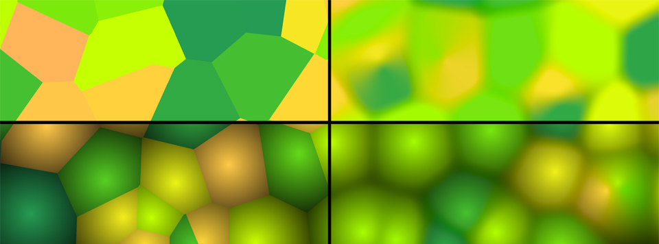
Left: traditional voronoi, Right: smooth voronoi