Motivation

---

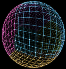
Everybody knows how to generate a polygonal sphere... but not everybody knows making good polygonal spheres. I mean, spheres that are usable for rendering with a rasterizer using, say, a texture, or a normal map. Often one resorts to the polar coordinates to construct the sphere and the texture mapping coords, since the polar coordinates are the natural parametrization of a sphere. The problem is that parametrization has singularities in the poles, and the mapping gets quite contractive (high derivative) on the surroundings of the poles, making it useless for texture mapping (the texture gets stretched a lot there). It also causes thin triangles to appear on the poles (unless a nonuniform sampling of the 2 parameters is used), as it can be noted on the image on the right. There are even more disadvantages with the polar parametrization; for example, it involves trigonometric functions, meaning that if one wants to compute tangents to the surface (for normal mapping for example) it has to resort to more trigonometric functions, that are usually too expensive to be abused on realtime shaders.

So, while the natural parametrization of the sphere is the polar one, we will probably want to use something else than the matematicaly obvious way of thinking. Here, we will use a piecewise algebraic parametrization (good for fast shader execution) that will suffer less parameter space distortion (good for texturing). On top of that, almost everybody having programmed a cubemap texture fetch is familiar with it.



The idea is simple, take a cube, and "normalize" it so each point on the surface is moved towards the center of the cube so that it's distance gets being one. In other words, generate a cube with many vertices, and normalize each of them. The trick will work of course with any concave shape, but a cube not being the simplest one (a thetraedra) is basic enough and it's very easy to manage.

For example, since each face of the cube has a simple (and natural) rectangular parametrization (0,1)x(0,1), we get automatically a simple parametrization domain for the sphere too. The rest of the article is about this parametrization, and to the way one can extract the corresponding tangent space basis vectors analytically, in an exact and cheap way, even per pixel if necessary.

The sphere description

---

We start by taking one of the faces of the cube (actually all the article will deal with one of the six faces, the other faces follow identical steps). For example the +z face (I assume OpenGL coordinate system, ie, the one you learn at school : x=right, y=up, z=towards you). Let's call the two parameters of the face surface domain s and t, with values in the interval [0,1]. We want our cube to be centered in the origin, and ranging on the [-1,1] values, so our surface points p are expressed as:

p(s,t) = ( 1-2s, 1-2t, 1 )

next we normalize this point on the surface of the cube to get a point q on the surface of the sphere:



meaning



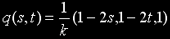
where   k² = 3 + 4(s² - s + t² - t)

that can be rewrite as



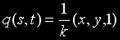
with

x = 1-2s    y = 1-2t    k² = x² + y² + 1

The inverse mapping   f: ℜ³ → ℜ² (the one that goes from q to parameter space) is equivalent to cast a ray with direction q into the plane z=1, and takes the form



and that's actually what I imagine the cubemapping units of the GPU do to fetch the texel data.

The real deal

---

Now that we understand what the sphere really is, it's time to compute its tangent space. Actually, we will compute a tangent space basis such that its basis vectors follow the texture coordinate parametrization, that's what you need to do normal/bump mapping. Basically, the surface tangent vectors will be aligned to the directional derivatives of the sphere (think about it as follows: when you slightly change s or t the point q moves, and the difference between the new and old position of q is your tangent vector. We could also be measureing changes with respect to x and y of course, so lets use those since they are easier to deal with. The derivative with respect to x will give a tangent u, and the derivative respect to y will give the second tangent v (sometimes called binormal). Now take care, these two vector will not necessarily be orthogonal to each other, although they will be linearly independant, will so define a tangent plane to the sphere, and will of course be orthogonal to the normal n to the surface.

We start the maths doing

q(x,y) = (x, y, 1) ⋅ (x²+y²+1)^-1/2

as before, and derivating repect to x and y to get u and v:

u=∂q/∂x and v=∂q/∂y

with

u = ∂q/∂x = ( ∂q_x/∂x, ∂q_y/∂x, ∂q_z/∂x )
v = ∂q/∂y = ( ∂q_x/∂y, ∂q_y/∂y, ∂q_z/∂y )

of course. So,



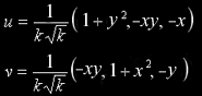
If only the direction of the tangent basis vectors are of interest (for example because the application needs normalized tangent space vectors), then one can skip the common factor to the three components. By replacing variables the expression gets simpler to code:

u = ( 1+y², -xy, -x )
v = ( -xy, 1+x², -y )

Note that these two vectors are not perpendicular (check for <u,v>≠0), although their cross product n = u⨯v = k²⋅(x,y,1) = k²⋅q(s,t), what means that points indeed on the direction of the surface normal n.

Implementation

---

Finally the implementation is easy, very few computations are needed, none of them complex. The image on the right shows the u and v vectors computed as just explained. Please note that these tangent vectors are exact, they are not based on differencing vertex positions or texcoords, they are analytically correct, what means that one can get per pixel exact tangent basis, if needed. In that case, one can move from the vertex shader down to the pixel shader s and t (only two floats, half interpolator!) and evaluate u and v, or perhaps compute those in the vertex shader and pass them to the pixel shader (6 floats...). Take also into account that u and v are not orthogonal to each other, so some tricks as transposing the tangent matrix will not work (you will have to compute the inverse, or better, do the bump lighting computations in object space!).