Intro

---

Very often you find yourself in the need to compute the distance to an isosurface that is defined through an implicit scalar field f(x). This happens in just too many situations, like in raymarching mandelbulbs or julia sets or any sort of regular distance fields, rasterizing functions or rendering 2d fractals, just to mention a few. In this article I'm going to explain the usual way to estimate a distance to the isosurface, and how that can help avoid one particular annoying issue that often arises when rendering procedural graphics - the compression and shrinking of your pattern.

The problem

---

Say you are using some random implicit function, and imagine we are using this function to draw some shape (defined by it's f = 0 isosurface). Let's take one simple formula as an example:

f(r,a) = r - 1 + sin(3a+2r²)/2

where, as usual, r = sqrt(x²+y²) and a = atan(y,x), meaning f is in the end of the day a function of regular x and y cartesian coordinates. This formula produces a simple 3-lobe fan shape, and it could easily be one of the many elements making a bigger procedural image/texture or something.

Now, if you were to do nothing special but just assign a color to each pixel based on the value of f, your first instinct would probably to thresholding the function with a smoothstep function:

This code produces an interesting image (see image to the left), but it's probably not what you want. You are probably looking for a constant thickness of the shape.

Perhaps you would be more interested in a constant thickness outline image, probably based on a more homogeneous scalar field. In fact, if you could compute some sort of distance to the zero-isoline of f, that would be great, wouldn't it? (now you probably see how this is related to doing distance based raymarching and you try to find intersections with the zero-isosurface). Perhaps, you would be interested in being able to compute an image like the one on the right. Let's see how we can achieve this!

The maths

---

Let's do some maths in order to understand the technique. The implementation is going to be terribly simple and you can skip this paragraph and go straight there, although I always think it's a good idea to understand what's going on behind the code.

So, we start by having a look at the distance field of our example function f. The image to the right of this text shows it in grey scale, on which I have mapped the values of f to a shade of grey such that f = 0 is represented in black and |f| > 0 shows a brighter color, through a pow() function for the purpose of making the f = 0 isoline more pronounced. Of course, in the interior of the shape f < 0 and in the exterior f > 0

Now, we are interested in computing the distance to our f = 0 shape at a given point in space x, which is represented by the yellow dot. The distance to the isoline is the distance to the red point, which is the closest point in the isoline to the yellow point. Let's call that closest red point x+e, such that e is the vector going from the yellow to the red one. What we are after here is |e|, the length of e, which is the distance from the x to the isoline/isosurface. In this setup, since x+e is in the 0-isoline, we clearly have

f(x+ε)=0

Let's assume we are pretty close to the shape, meaning, that |e| is small. Then, we can expand f(x+e) in its Taylor's decomposition

f(x+ε) = f(x) + ∇f(x)⋅ ε + O(|e|²)

where the dot (⋅) means dot product, as usual (remember that both the gradient and e are vectors here). If we were close enough, indeed, then we could just use this linear approximation of f and say that

0 = |f(x+ε)| ≈ |f(x) + ∇f(x)⋅ ε|

meaning that

0 ≥ |f(x)| - |∇f(x)⋅ ε| ≥ |f(x)| - |∇f(x)| ⋅ ε

the first inequality being due to the triangle inequality, and the second one to the basic properties of dot product. From there, we could isolate

which gives us an upper bound to the estimated distance from x to the zero-isosurface of f.

Another way to arrive to the same results would be to construct a plane tangent to the surface at x+e, defined by the gradient/normal of the surface, and intersect a line going through x that is parallel to the gradient/normal with the plane.

Distance field for f(r,a) = r - 1 + sin(3a+2r²)/2

Note the dark spiral that leaves from the 3 spikes of the main shape, that explains their elongation when f() was rendered by direct color mapping in the first image in the header of the articles.

The implementation

---

All we need is the gradient of f(x). In the case of the function in the example above, we'd have the following code:

which you could combine in a single function in order to reuse some of the terms.

However, in most of the times we won't have an analytical gradient vector of our function f, so we are forced to do a numerical approximation with the regular central differences method

(which can be done with three samples only or using dFdx(x) and dFdy(x) if you don't care about precision too much) and then use the formula above to compute the distance estimation (de in the code) to compute the color as before:

This method evaluates f four extra times, which makes it more expensive. Besides, choosing the right value for h might be difficult sometimes. But more often than not, it simply works pretty well. When analytical gradients can be computed, it is strongly recommended to use them instead, like when rasterizing 2D fractals or raymarching mandelbulbs or julia sets.

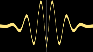
Plotting 1D functions with constant thickness

---

This method shines for approximating distances to smooth 1D functions. Say we have a function f(x) we want to plot in an implicit fashion (as opposed to explicitely by rasterizing lines). Then we can construct the implicit function g(x,y) = |y-f(x)| and to plot that directly, for example by selecting only the pixels where g(x,y) < thickness. That works great, except that soon enough we'll notice that the graph gets uneven thickness, something like this:

Here the flat parts of the graph are the thickness we want, but the step ones are too thin. The problem is that if we increase the thickness parameter, then we get the middle of the graph to look okey, but the flat areas are too thick, like this:



So, here's where we want to apply our gradient based distance estimation method:

∇g(x,y) = (1, f'(x))

and from there we can compute our distance estimation to f(x) as



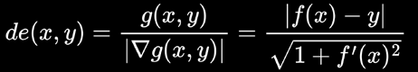
When we use that to plot, we get a pretty uniform thickness across the function:



We can interpret the formula as computing the distance to the tangent line to the graph at each point, which has slope f'(x).

And this is a realtime version of if, in case you want to play with it and see how it behaves: https://www.shadertoy.com/view/mt3SDN.

The example

---

This is a shader with source code available (click in the title bar) with the implementation of this idea.