


Intro
Back in 2007 I made two 4 kilobyte demos that requrired polygonal mesh compression, Stiletto and Kinderplomber. One featured skeletal mesh deformation of a part of a female body, and the other one did some global illumination on an asbtract tree shape. Both meshes were organic shapes, and were compressed in a few hundred bytes by using (two different) subdivision methors to amplify the data set, and also by heavily comrpessing the low resolution base mesh. The compression methods were an evolution of the naive method used for the 64 kilobyte demo Paradise. This article is about the compression methods used in those two intros.

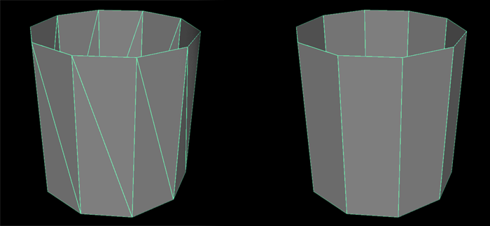
Mesh for Kinderplomber, compressed down to
967 bytes (2.04 bytes per triangle)

Mesh for Stiletto, compressed down to
710 bytes (1.75 bytes per triangle)
Step 1 : data input and data output
The first step is setting the rules of the game. The rules in these 4 kilobytes demos where:
- The meshes are going to be really low resolution
- Meshes are made of quads, not triangles: triangles are efficient for rendering, but they usually bring little additional geometrical information for most organic surfaces.
- There is an entropy compressor processing our data (probably an arithmetic encoder).
Modeling with quads: modeling with quads not only is convenient for the subdivision routine, but also is more efficient into representing surfaces. Usually the extra edges introduced by triangulating surfaces brings little to no extra geometrical information, at the cost of having more topological (connectivity) information to store.
Entropy compressor: this is very important and often misunderstood. Assuming
our data streams are going to be encoded with some arithmetic encoder or some
other sort of entropy compressor (ZIP, PNG, Crinkler, Kkrunchy, UPX...), it is a bad
idea to try to be too smart in our end and pack data streams that are unrelated to each other.
Suppose you have per vertex positions x, y and z, and also per vertex colors and UV texture coordinates. Say that your x, y and z values have been quantified to 6 bits each, the RGB colors to 6 bits per component too and the UVs to 6 bits for U and 6 bit for V. Your compressed vertex format aligns nicely to 48 bytes, and so you decide to store the data in this "compact" form. You might even decide to delta encode the vertex data (an array of structs) hoping to help the compressor. This is a mistake. The redundancy of the data happens across sample point of the same data channel. And by packing the data in a satisfying layout, you are shuffling the data and confusing the entropy compressor. Instead, store your data as a struct of arrays, and let each individual data channel (X, Y, Z, R, G, B, U, V) be serialized independently so that the entropy compressor can explode the coherency of the data values.
This brings us to a second consideration. Because data packing doesn't need to happen anymore, you don't need to limit yourself to any particular number of bits per channel. Or if you do, you should not take data aligment considerations into account, but only signal to noise / quality / compression ratios.
For example, if after quantification the X component of vertices happens to range from 0 to 41, do not try to store it in a 6 bits variable. Store it simply in a integer, or whatever is big enough to store it, and let the arithmetic encoder use the 5.4 bits it takes to store numbers from 0 to 41 (in the worst case scenario that all these numbers are pure random).
In a similar fashion, do not RLE encode your data. Do not interfere with the compressor, just present the data to it in the most simple way you can.
Step 2 : quantification
When it comes to quantify the vertex positions into an integer, we are all always tempted to use a power of two as the number of subdivisions. For example, we like to encode each axis of our model into 256 values, or perhaps 4096. Generally this leads to non optimal bit rates. For two reasons:
First, each axis probably needs its own quantification scale. Assuming that, as explained above, the size of each data stream (in bits) doesn't need to match the others (cause there no longer is packing constrains), there's no reason not to use 8 bit for the x and z component of the vertices and 12 bits for the y, if you are compressing the model of a tree.
Furthermore, you should not chose your number of bits beforehand. Instead, what you want is to limit the max error you allow in the quantification, and then, based on the bounding box of the object, decide how many divisions or cells you need in each dimension. This will create a grid or regular cubes (as opposed to boxes) with no wasted quantification in any axis.
When doing so, of course, the number of segments in each dimension will no longer be a power of two in general. But that is simply not a problem. Rememeber the entropy encode is not limited to integer number of bits per value, so it will be no more efficient in encoding non-power of two number of steps. In general, the formula you want to use to decide the amount of segments for quantify your 3d model based on its bounding box, obviously:
So, for example, if your model is 7 meters wide, 3 meters tall and 2 meter thick, and the error you want to allow is of 1 centimerer maximum, then the number of segments will be 700, 300 and 200 in each dimension, and the amount of bits used to encode each dimension will be 9.45, 8.22 and 7.64 respectivelly.
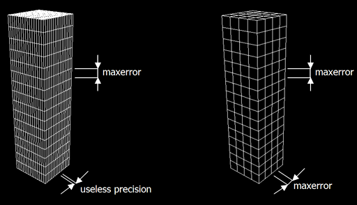
Left: bad choice of number of segments per coordinates, due
to an attempt to satisfy a rounded power-of-two number of segments.
Right, correct choise of number of segments per coordinate based
on the length of bounding box in each dimension and maximum error
desired in the quantification
Step 3 : codification
There are many ways to encode the geometry and connectivity of the mesh. I'll describe the methods I used in Paradise, Kinderplomber and Stilletto, which are improvements of the method right before it. The metric to compare the different methods is the number of bytes required to store the model normalized to the number of triangles in the model (2 per quad):
Method 1 (Paradise) - 2.8 bytes per triangle
This is the baseline, no effort is really done into exploiting redundancy, except for separating each data channel in a different stream:
- for each vertex
- write the x coordinate
- for each vertex
- write the y coordinate
- for each vertex
- write the z coordinate
- for each quad
- write vertex 0 ID
- write vertex 1 ID
- write vertex 2 ID
- write vertex 3 ID
Method 2 (Kinderplomber and 195/95/256) - 2.4 bytes per triangle
Some (poor) geometric redundancy is extracted by computing vertex deltas (difference between the current vertex being encoded and the previous one). The connectivity is still raw data (in streams):
- for each vertex
- write the difference of x coordinate with respect to the previous vertex
- for each vertex
- write the difference of y coordinate with respect to the previous vertex
- for each vertex
- write the difference of z coordinate with respect to the previous vertex
- for each quad
- write the difference of vertex 0 ID with respect to previous vertex ID
- write the difference of vertex 1 ID with respect to previous vertex ID
- write the difference of vertex 2 ID with respect to previous vertex ID
- write the difference of vertex 3 ID with respect to previous vertex ID
Method 3 (Stiletto) - 1.8 bytes per triangle
The method in Stiletto was the most complex of all. Since geometry and connectivity are related (vertices connected together by and edge are likelly to be closer to each other that vertices that are not connected by an edge), I chose to encode both simultanteously (but not together). The first step was to segmentate the mesh in quad-strips (a series of connected quadrilateral). Each quad in the strip requires only 2 vertexID rather than 4 (except for the first one of each strip). As the strips are iterated, the vertex IDs are output and also the vertex coordinates. If the vertex is a new one, it is simply output. If the vertex has been serialized before (perhaps by another strip), then only the connectivity is stored, but not the vertex coordinates (and data). Therefore there's one stream of vertex IDs for connectivity, one stream of binary flags of visited/unvisited vertices, and then as many streams of vertex data as channels are in the vertex format.
On top of that, instead of using a simple delta coding of vertex coordinates (the context of the delta being different for each data channel in the vertex format), Stiletto used parallelogram prediction schema, where each polygon is assumed to be close to a parallelogram (where D-C = B-A), and only the deviation or error is encoded (e = D'-D):

With all the pieces together, the encoging steps are as follow:
- for each strip
- write length of strip
- for each strip
- encode( vertex 0 )
- encode( vertex 1 )
- each quad in the srip
- encode( vertex 2 )
- encode( vertex 3 )
- write vertex visited
- if vertex visited
- write vertex 0 ID
- else
-
- write vertex coordinate x error from parallelogram
- write vertex coordinate y error from parallelogram
- write vertex coordinate z error from parallelogram

Overall the code complexity is a little bit bigger than the first and second method, but the gains are important. Compare how the old and new method encode the same 11 polygons:
Method 1:
quads: { 0, 1, 2, 3, 2, 3, 5, 4, 4, 5, 7, 6, 6, 7, 9, 8, 8, 9, 11, 10, 12, 13, 15, 14, 14, 15, 17, 16, 16, 17, 4, 18, 18, 4, 6, 19, 19, 6, 8, 20, 20, 8, 10, 21 }
Method 2:
quads: { 0, 1, 1, 1, -1, 1, 2, -1, 0, 1, 2, -1, 0, 1, 2, -1, 0, 1, 2, -1, 2, 1, 2, -1, 0, 1, 2, -1, 0, 1, -13, 14, 0, -14, 2, 13, 0, -13, 2, 12, 0, -12, 2, 11 }
Method 3:
visited: { 0,0,0,0,0,0,0,0,0,0,0,0,0,0,0,0,0,0,1,0,1,0,1,0,1,0 }
strips: { 5, 7, 9, 11 }
The method 3 not only is shorter, but the stream of "visited" is going to be encoded in less that one bit. So basically, with the third method the conectivity becomes pretty much irrelevant in comparison with the encoding of the geometry.