


Intro
IFS (Iterated Function Systems) produce some of the best known fractal images, like the famous Berensley fern. They have been used for image compression, but more frequently especially in the 90s, as a method to create nerdy posters and wallpapers.
I made my first IFS images back in 1998 in basic, but later on I wrote a simple C program that could render high resolution images, like these ones below, that were in fact computed at 6000x9000 pixels with 2x2 antialias (12000x18000 effective sampling points). One of them made it into the finals of a fractal image contest, and the other one was used as background for a cover of a book, but that's another story.

Really understanding the maths of IFS is not necessarily easy, but implementing it is amazingly simple. The images are the attractors of the actual iteration of functions. The functions are just linear functions, affine transformation T if you want, that take a point p and transform it into p' with rotation, skew and scale factor A and a translation B:
T(p) = A⋅p + B
that can also be written as
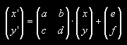
When applying T to all the points of a plane (an image if you want) this gets expanded or contracted, and that contraction factor is just the determinant of A (since the transformations are linear), as usual.
contraction = |A| = ad - bc
For rendering all the IFS images in this site I only used four such transformations, but you can choose any number. We will be applying these transformations to points in the plane, and assuming the overall transformation is contracting, the iterative process will make the complete plane converge to a given set, the final image. The geometry of this set, the attractor of the IFS, is usually fractal, even if the transformations are linear, but that's out of the scope of this little article.
The iterations happened like this: pick a random point in the plane, one of the four transformations at random, and apply it. This gives a new point. Now, pick again one of the four transformations at random, and apply it again. Repeat, few thousand millions of times.
pn+1 = T(pn)
This will give an "orbit" for that very first starting point we chose. The chaos game theory ensures that if the average contraction factor is less than that one, we will get not a random point cloud neither an exploding orbit, but an well defined shape, the attractor.
Well, for this to be true, chaos theory and symbolic dynamic mathematics say that you must randomly choose the transformation from the transformation set of the IFS. This way, the orbit densely overlaps the attractor. In the other hand, to help the chaos game converge faster, it is better not to randomly select a transformation from the transformation set of the IFS, but with a probability proportional to the area covered by this transformation over the total area of all the transformations:
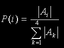
To make things more interesting, it is also possible not to only record the attractor, but also the density of the attractor. This can be interpreted as the probability of the iteration to step at a given point across the orbit. After selecting the probabilities according to the equation above, this density over the attractor should be quite smooth.
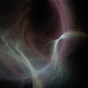
IFS, "Flames" style
A variation of the IFS fractals became popular in the 90s through the software called "Flames", which added a non-linear deformation to the regular IFS method and added colors to the IFS plots. This is an example of a random IFS of four transformations rendered with a nonlinear transformation and color in the "Flames" style:
Source code: https://www.shadertoy.com/view/4dXGWS
So, the technique is based on applying a nonlinear transformation after the affine map, before accumulating the orbit on the plane. It is important to note that to keep the convergence of the orbit unaltered, the space compression/expansion produced by these nonlinear transformations should be taken into account at the time of computing the probabilities assigned to each of the functions in the IFS. However, unlike affine maps which are linear and have constant derivatives/Jacobian (equal to their determinant), the nonlinear transformations Jacobian (space deformation compression/expansion rates) are functions of p themselves, so they cannot be precomputed. That means we can no longer pre-compute probabilities before starting the IFS iterations. So usually, rather than recomputing such probabilities in each iteration of the orbit, we simply ignore it. Meaning, we do not take the non-linear transformations into account when computing our IFS probabilities. And that is okey in many cases, although not optimal.
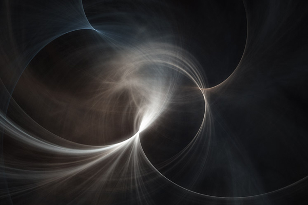
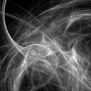
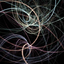
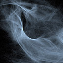
Anyways, coming back to talking of less technical things, in order to create the images at the top of the article, the nonlinear transformation was a rotation in which the rotating angle was proportional to the signed horizontal distance from the point to the origin.
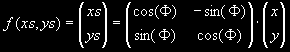
Additionally, a sinusoidal component was added to this angle that changed each iteration.
φ(pn) = |pn| + sin(ω⋅n)
I call this deformation "Twist". Adjusting the frequency and amplitude of this sinusoidal component, the thickness and intensity of the "arcs" on the picture can be adjusted. Without this variation, the arcs would become just "threads".
But any other transformation will work too. For the video above with the red IFS animation, an plane inversion was used, where
F(p) = p/|p|2
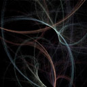
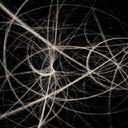
And the following images below were created around 2001 by randomly choosing affine maps and using the simple twist nonlinear transform. Because it was 2001 though, this was implemented in the CPU and took a few hours to render. You can click on them to see a higher resolution version:


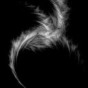
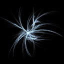
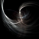
I wrote a small application that randomly created thousands of IFS images. To quickly discard those transformations creating disperse attractors, the application only used those random transformations with a contracting coefficient smaller than 1.5. These images were, of course, low-resolution and low quality (low number of iterations). The very first two images in this page were created by choosing from this collection of random images.
For example, to make the first image, I chose one of the random images I liked, and worked on it. It's color was decomposed in the hue and its intensity. As explained, the iterative process does not just show the attractor, but its density. So, for the color intensity, the density of the attractor was chosen. In fact, it is the square root of the density normalized to the maximum/minimum value over the image. The square root was not chosen for any mathematical reason; it was just used to adjust the contrast of the image in the image-synthesis part (where the colors are kept in floating point), to avoid crappy manipulation in Photoshop using 8 bit precision.
The color was a bit more complicated to create. Actually, it stores important information about the dynamics happening on the attractor: each point in the attractor is accessed from another given point of the attractor by the application of one of the transformations used, his "preimage" (if these transformations overlap, there is more than one preimages exist). In other words, each point in the attractor can be identified by the symbolic sequence of transformations used to get that point from the original one. This sequence is called the "address". This address, expressed in the correct base (four in my case, because I selected four transformations), defines a number between 0 and 1. The coloring of these images was done based on that number. Each new point on the orbit generated a color based on his actual address, and then accumulated on the plane.
To get a color based on the address of a point, a sinusoidal function was used for each color component (red, green and blue), for example the following one, although any other will for just fine, as explained in this article.
color = vec3(0.4,0.6,0.7) + 0.25*sin( address + vec3(0.5,0.9,1.3) )
Finally, a "glowing" postprocess effect was done to enrich the visual quality. This effect is responsible for the light emission effect on some parts of the image (the brighter ones). To get it, the image was low-pass filtered (a gaussian filter) and added back to the original image in a 50% proportion.